Measurement of atmospheric electric fields

1. INTRODUCTION

The local voltage in a space can be measured with an electrostatic fieldmeter either earthed to act as a potential probe [1,2] or arranged as a voltage follower probe [3].

The ambient atmospheric electric field E_a is conveniently measured using an electrostatic fieldmeter at earth potential mounted on a pole a known distance above ground level. In this arrangement the fieldmeter is being used as a probe of the local potential at its mounting height. This mounting arrangement is simple to implement, avoids anxieties about ground level dust, debris and insects entering the fieldmeter sensing aperture and gives useful enhancement to the basic fieldmeter sensitivity.

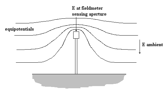
The electric field at the sensing aperture of an earthed fieldmeter E depends on the local potential V, present at that position before the fieldmeter was introduced, and the effective diameter of the fieldmeter d, as:

E = a V / d

The factor a is near unity. The fieldmeter needs to be several diameters away from nearby surfaces. This approach is very appropriate for measurement and for long term continuous monitoring of atmospheric electric fields.

A fieldmeter used as a potential probe provides the opportunity to measure atmospheric electric fields. This is particularly relevant to assessment of the local risk of occurrence of l ightning - see for example descriptions of the JCI 501 and JCI 503 systems and the paper presented at the ESA meeting at Niagara Falls in 2000.

2. VERTICAL ATMOSPHERIC ELECTRIC FIELD

2.1 Introduction

The sensitivity of a fieldmeter as a potential probe, mounted well clear of nearby surfaces, is close to:

V = E_fm d / a

? where E_fm is the electric field (V m^-1) at the fieldmeter sensing aperture responsible for the fieldmeter reading and d the effective sensing head diameter (m).

For an ambient atmospheric electric field, E_v (V m^-1) the local voltage at a height h (m) is:

V = E_v h.

Hence the ambient electric field is obtained from measurement of the electric field at the fieldmeter sensing aperture as:

E_v = E_fm d / h

There will be a contribution to the electric field measured dependent on the alignment of the sensing aperture relative to the ambient electric field. If for example the two field components are in directions to add, then the atmospheric field can be derived as:

E_v = E_fm d / (h (1-d/h))

As d/h is normally small the influence of this effect is small.

&nb sp;

2.2 Validation of sensitivity

The actual sensitivity of measurement of a fieldmeter acting as a potential probe can be checked in-situ by applying a calibration voltage to the whole fieldmeter and mounting assembly. This gives the fieldmeter reading as a function of local voltage - so the local ambient atmospheric electric field is obtained knowing the mounting height of the sensing aperture. Such calibration measurements need o be done under electrostatically stable atmospheric conditions. This probably means a clear blue sky and no nearby sources of smoke or dust.

Where the fieldmeter is mounted other than above a large plane ground area well clear of any buildings or earthy projections there will be need to ?interpret? electric field measurements in relation to the geometric arrangement of the surroundings. This can be done with computer modelling calculations - but this may be difficult and lacking conviction in complex three dimensional arrangements. One approach to tackle this problem is to normalise readings in relation to otherwise known ambient atmospheric electric field values with, for example, a clear sky situation - when the ambient field is typically around 100V m^-1. The actual value needs to be checked at the same time somewhere nearby.

If the ?earth? around the fieldmeter mounting is not flat, or there are local perturbing items, then the ?height? about earth may be ambiguous. In this situation it will be best to measure the local atmospheric electric field from the difference in potential for a known change in height. The value obtained may then be used to normalise height measurements.

2.3 Operational health monitoring

Application of a modest level alternating potential to the fieldmeter assembly can be used for continuous monitoring of the operational health of the observation system. This ensures confidence in observations during operation in adverse environmental conditions.

2.4 Practical measurements:

The above discussion illustrates basic arrangements for measurement of atmospheric electric fields. It is directly appropriate for measurements with fieldmeter instruments that have the ability to provide continuous measurements even through periods of heavy rain [4]. An appropriate fieldmeter for such measurements is the JCI 131 electrostatic fieldmeter. This instrument has been designed, constructed and used for reliable long term continuous operation even in very wet environments and with driving rain [4,5,6].

The advantages of an upward looking fieldmeter for long term continuous observations is simplicity of mounting and the use of rain to keep the surfaces of the sensing region clean. If such instruments are not ava ilable and the environment will not be too adverse then good quality measurements may be made using more standard fieldmeters mounted with the gallows type structure sketched below.

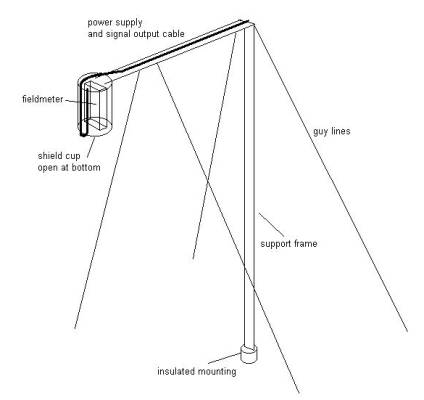
The fieldmeter sensing aperture is protected from direct impact of rain by pointing downwards. The fieldmeter case, circuits and connections are protected by mounting the fieldmeter up into the deep up-turned cup. Dry air purging of the fieldmeter circuits and sensing region may be desirable. If the cables are routed down the inside of the cup, and then back over the outside, then it is wise to wrap them in a conducting shield (e.g. aluminium foil) connected to the cup and ?earth? of the fieldmeter to avoid risk of any residual charge on the cable insulation affecting readings. The mounting structure should be conducting and connected to the ?earth? terminal of the fieldmeter. It is adviseable to mount the support structure and any guys with insulation at their ground level ends. This allows calibration voltages to be applied to the whole assembly for checking system measurement sensitivity (as noted in Section 2.2 above) with minimum risk of interference to measurements from static charge retained on insulating surfaces.

3. HORIZONTAL ELECTRIC FIELD COMPONENT MEASUREMENT

3.1 Introduction

Horizontal electric fields can be measured using two fieldmeters to measure the difference in potential over a known horizontal separation distance. Four fieldmeters positioned north, south, east and west would for example provide opportunity to determine the bearing of the charge centres of moving thunderclouds. Such measurements have relevance in determining the direction, movement and strength of electric fields from thunderclouds, hurricanes, erupting volcanoes, etc. The relation of local vertical and horizontal electric field components to the quantities of charge and their altitude and distance of thunderclouds may be modelled with Spreadsheet calculations treating the cloud charges, and their image charges below the ground plane, as dipoles.

Where measurements are made only a few meters above the conducting surface of the earth the horizontal field components are low - and will be very much less than the vertical component. To avoid signals arising from cross coupling of the local vertical field component to horizontal observations it is important that the two fieldmeters for measuring the horizontal are exactly the same effective height.

The arrangement suggested for reliable measurement of horizontal components of atmospheric fields is to mount 2 or 4 fieldmeters at either ends of a rigid cross arm structure. This might be a linear cross arm for mounting two fieldmeters or two interconnected cross arms at right angles for mounting 4 fieldmeters. The cross arm assembly is mounted at the top of a vertical mast so that it can be rotated about an axis at right angles to the plane of the cross ar ms. The assembly is insulated from earth and voltages can be applied for calibration of the local voltage sensitivity of the fieldmeter instruments. The vertical component of atmospheric electric field is then obtained from the average of the 2 or 4 fieldmeter readings and the horizontal components by the NS and EW differences.

3.2 Measurement arrangements

As noted above, a fieldmeter acts as local potential probe. For a fieldmeter with a body diameter of, say, 100mm (e.g. JCI 131) the voltage sensitivity is close to 10V m^-1 per 1V of local potential can be expected. The exact relation between output signal and local potential for individual instruments is established by measuring the change in output in response to a known change in the potential of the fieldmeter system (see Section 2.2 above). The noise level and zero stability of individual JCI 131 fieldmeters is about 1V m^-1 so the limiting of local voltage measurement is about 0.1V. For a 2m cross arm length the resolution for horizontal field observations is then likely to be say 0.1V m^-1.

Ambient vertical electric fields may be a few kV m^-1. For a field of say 2kV m^-1 and a height of say 2m the local potential at the fieldmeters would be 4kV. There are two features that arise from this: first, that measurement of local voltages at multiple fieldmeters hence needs a measurement resolution around 10^-4. Second, a difference of local voltage between fieldmeters of 0.1V is equivalent to a height difference of only 0.05mm.

To achieve best resolution for difference signals it is appropriate to arrange to adjust the voltage of the fieldmeter assembly to the average of the local voltages observed by the fieldmeters. This can be done using a servo system that adjusts the voltage of the fieldmeter assembly to minimise the average of the fieldmeter signals. The fieldmeters can then operate on their most sensitive range, and so provide best signal to noise performance. The average local voltage is obtained from the sum of the servo voltage applied and the average of the fieldmeter observations.

3.3 Preparation for practical measurements

It is best to make the following system tests on a large flat open area with stable atmospheric electrostatic conditions. This requires clear ?blue sky? conditions with no nearby sources of smoke or dust.

The following approach is suggested:

- mount the fieldmeters as symmetrically as possible at either end of the cross-arm with this mounted at right angles to a vertical mast that can be rotated in good quality bearings with minimum radial clearance and good mechanical stability. A preliminary test of the mounting maty be made by checking the mechanical height of fieldmeter casings as the assembly is rotated.

- mount a precision tiltmeter on the cross arm.

- adjust the alignment of the mast axis so that there is no change in the tiltmeter reading at rotation of the mast. The axis is now vertical. (An angular accuracy of ½ minute of arc is equivalent to an accuracy of 0.2mm in relative vertical position of the two fieldmeters on a 2m cross arm).

- Calibrate the voltage sensitivity of the fieldmeters by applying a calibration voltage to the mast. This is best done with a step function application and removal of calibration vo age so that changes in output can be measured reliably, even if atmospheric electric field conditions are not fully stable.

- Check that rotation of the fieldmeter assembly, to interchange the positions of the fieldmeters, leaves the readings of each fieldmeter stable. If it does not it may be that the mast is not adequately vertical or the electrostatic environment is not fully symmetrical. The reading of the tiltmeter ?zero? is noted.

- Differences between fieldmeter readings will now be due to differences in their heights. Actual height correction factors may be calculated from interpretation of fieldmeter readings to give the vertical component of electric field values. It is useful to check that the difference signal observed with a slight defined tilt of the axis of rotation matches that expected from the titlmeter angle and the height offset adjustment applied.

- The difference signal between the fieldmeters, taking account of their individual sensitivities, should be independent of the calibration voltage applied to the mast structure.

References:

[1] J. M. Van der Weerd "Electrostatic charge generation during washing of tanks with water sprays, II Measurements and interpretation" Static Electrification Conference, London, 1971 Institute of Physics p158

[2] J. N. Chubb, G. J. Butterworth, "Instrumentation and techniques for monitoring and assessing electrostatic ignition hazards" Electrostatics 1979

Inst Phys Confr Series No 48 1979 p 85

[3] R. E. Vosteen "Electrosta tic Instruments" International Conference on Charged Particles - Management of Electrostatic Hazards and Problems, Oyez 1982

[4] J. N. Chubb ?Experience with electrostatic fieldmeter instruments with no earthing of the rotating chopper? 'Electrostatics 1999' Conference in Cambridge, March 29-31, 1999. Inst Phys Confr Series 163 p443.

[5] "A system for the advance warning of lightning" Pa per presented at the Electrostatics Society of America 'ESA 2000' meeting, Niagara Falls, June 18-21, 2000

[6] J. N. Chubb and J. Harbour ?A system for the advance warning of risk of lightning? Paper presented at Electrostatics Society of America Annual meeting at Brock University, Niagara Falls June 18-21, 2000

| Home | News | Products | Specifications | Papers | Meetings | Contact JCI | Sitemap |

For best results view these pages with a Netscape Navigator browser.

John Chubb Instrumentation,
Unit 30, Lansdown Industri al Estate, Gloucester Road, Cheltenham, GL51 8PL, UK
Tel:+44 (0)1242 573347 Fax: +44 (0)1242 251388
email: jchubb@jci.co.uk

Page Update: 08/10/2004 © John Chubb Instrumentation.